Kernels
Gaussian process를 구현할때에는 kernel을 지정해야한다. Kernel은 Gaussian process random variables의 covariance를 의미한다. Mean function과 함께 Gaussian process를 완전하게 정의하기 위해 반드시 필요한 요소이다.
Gaussian process(GP)를 사용할때에 어떤 kernel(covariance function)을 선정해야 할까?
GP model을 구현할때에는 GPML(for MATLAB), GPy(for Python) package들이 주로 사용되는데, 이 package들에는 default kernel이 설정되어 있지 않다. 그 이유는 어떤 kernel을 사용하냐에 따라서 GP model의 generalization properties가 결정기 때문. 문제를 해결하려는 사용자가 직접 문제에 적절한 kernel을 지정해야 하는것이다.
“Support Vector Machine 문제를 해결하기 위한 kernel?”
Standard Kernels
Squared Exponential Kernel
Squared exponential kernel은 GP나 SVM 문제에 default kernel로 활용된다. RBF(radial basis function) kernel로 다음과 같이 정의할 수 있다:
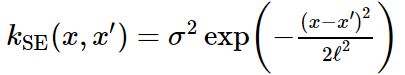
- lengthscale ℓ : It determines the length of the ‘wiggles’ in your function. In general, you won’t be able to extrapolate more than ℓ units away from your data.
- output variance σ^2 : It’s just a scale factor. It determines the average distance of your function away from its mean. Every kernel has this parameter out in front.
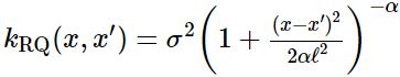
Rational Quadratic Kernel
여러 squared exponential kernel들이 다른 lengthscale로 더해지면 rational quadratic kernel을 얻는다. 그래서 이 kernel로 구현된 GP에서는 다양한 lengthscale에 대해 완만하게 달라지는 function들을 확인할 수 있다. 이 kernel에서는 parameter α가 large-scale과 small-scale variation의 relative weighting을 결정하다.
다음 rational quadratic kernel 함수에서 α –> ∞의 경우, squared exponential kernel과 동일해지는 것을 볼 수 있다.
보통 classification model이나 GP regression model을 setup하는 경우, squared exponential 또는 rational quadratic kernel을 사용한다.
이 두 kernel들을 통해서 “smooth”한 function들을 interpolating하고 대체로 쉽게 솔루션을 찾을 수 있지만, function들의 first few derivatives에 discontinuity가 존재한다면, 달라진다. 이런 경우 lengthscale이 매우 짧아지거나, posterior mean이 대부분의 영역에서 0이 되거나 또는 “ringing” effect를 갖게 될 수 있다. 이런 “hard” discontinuities가 존재하지 않더라도, lengthscale이 function에 가장 작은 “wiggle”로 부터 결정될 수 있다. 결국, data내 하나의 작은 non-smooth region이 존재하면, 다른 smooth region에서도 extrapolate할 수 없어진다.
만약 data가 2D 이상이라면, 이런 discontinuity를 인지하기 어렵다. 이런 경우, data를 더 넣을 수록, maximum marginal likelihood로 선정된 lengthscale이 끊임없이 계속 줄어든다. (“model misspecification”발생)
Periodic Kernel
똑같은 부분이 반복적으로 발생하는 형태의 function들을 model하기 위해서 periodic kernel을 활용할 수 있다. 이 kernel의 parameter들은 쉽게 해석가능한편이다.

- The period p simply determines the distance between repititions of the function.
- The lengthscale ℓ determines the lengthscale function in the same way as in the squared exponential kernel.
Locally Periodic Kernel
Periodic하지만, 시간이 갈수록 변경하는 (varying over time) function을 model해야하는 경우, locally periodic kernel을 활용할 수 있다. 다음과 같이 periodic kernel와 squared exponential kernel의 product이다.

Linear Kernel
간단한 Bayesian linear regression을 구현하기 위해서는 linear kernel을 GP에 활용할 수 있다.
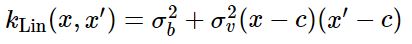
Linear kernel은 ‘non-stationary’하다. 이 점이 다른 kernel과 다른점인데, stationary covariance function들은 its two inputs의 절대적인 위치가 아닌 상대적인 position에 의존한다. 그래서 linear kernel의 parameter들은 origin을 specify하는 것이 key point이다.
- The offset c determines the x-coordinate of the point that all the lines in the posterior go though. At this point, the function will have zero variance (unless you add noise)
- The constant variance (σ_b)^2 determines how far from 0 the height of the function will be at zero. It’s a little confusing, becuase it’s not specifying that value directly, but rather putting a prior on it. It’s equivalent to adding an uncertain offset to our model.
Combining Kernels
Data가 모두 same type이 아닌 경우에는 위에서 설명한 standard kernel을 단일로 사용할 수 없다. Data에 여러 types of features가 존재한다면, 여러 kernels를 통합해서 data를 regress할 수 있다. 이렇게 different types가 포함된 data를 model하기에 적합한 kernel은 가장 기본적으로 multiple kernels를 서로 곱해서 확보할 수 있다.
Multiplying Kernels
두 개의 kernel를 통합하기 위해, 특히 이 둘이 서로 다른 input로 정의되어 있다면, 가장 기본적인 방법은 이 둘을 서로 곱해주는 것이다. 대략적으로 ‘AND’ operation을 수행하는 것으로 보면 된다. (즉, 두 kernels를 곱해서 얻는 resulting kernel이 높은 값을 가질 경우는, 각각의 kernel이 높은 값을 가지고 있는 경우이다.)
Linear times Periodic
[linear kernel] X [periodic kernel] = [periodic function with origin에서 멀어질수록 증가하는 amplitude]
Linear times Linear
[linear kernel] X [another linear kernel] = [quadratic function]
이 방식으로 any degree의 Bayesian polynomial regression을 구현할 수 있다.
Multidimensional Products
단 하나의 input dimension에 의존하는 두 개의 kernels를 곱하면, results = a prior over function that vary across both dimensions.
function value f(x,y) is only expected to be similar to some other function value f(x′,y′) if x is close to x′ AND y is close to y′.

Adding Kernels
두 개의 kernels를 더하는 것을 ‘OR’ operation을 수행하는 것과 동일하다. (즉, 두 kernels를 더해서 얻는 resulting kernel이 높은 값을 가질 경우는, 두 kernels 중 적어도 하나가 높은 값을 가지고 있는 경우이다.)
Linear plus periodic
[linear kernel] + [periodic kernel] = [periodic function with origin에서 멀어질수록 증가하는 mean]
Adding across dimensions
단 하나의 input dimension에 의존하는 두 개의 kernels를 더하면, results = a prior over functions which are a sum of one-dimensional functions, one for each dimension.
f(x,y) = f(x) + f(y)

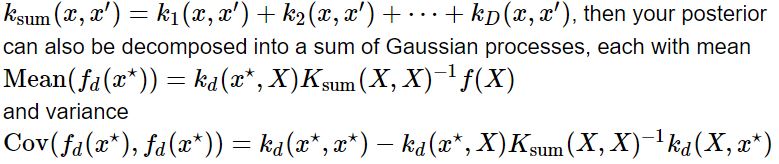
Additive decomposition
이러한 addition operation을 deocomposition을 위해 활용할 수 있다 - decompose the posterior over functions into additive parts.
Tips
Gaussian process와 SVM을 위한 kernels에 대한 정보가 매우 많음. 매우 comprehensive한 자료:
- chapter 4 of the book ‘Gaussian Processes for Machine Learning’ : http://gaussianprocess.org/gpml/
- documentation for the python GPy library : https://gpy.readthedocs.io/en/latest/tuto_kernel_overview.html
References
- The Kernel Cookbook : https://www.cs.toronto.edu/~duvenaud/cookbook/
- GPy : A Gaussian Process framework in Python (provides practical guide with lots of examples): https://gpy.readthedocs.io/en/deploy/